2.1. Relationship between potential energy and equivalent normal stress

Stresses in the lithosphere are due to forces acting on the lithosphere. These forces can be expressed as gradient of a potential energy. The potential energy per area of a dynamic topography h_d, i.e. the energy required for lifting up the entire lithosphere of thickness t_L by an amount h_d-h_d,0 is

The reference level for the potential energy is hereby chosen such that it has zero average over the surface of the Earth. In this way, the global average of the resulting scalar lithospheric stress anomaly (as defined in the main text) is also zero.

The second identity follows from Eq. 2 of the main text. With the definition given in the main text, it follows that the downhill force per area is equal to . Since the lithosphere is treated as a thin layer with no variation of properties with depth, it makes no difference whether the potential energy is due to dynamic topography or any other topography - a given potential energy will always cause the same stress field regardless of its origin.

In analogy to Eq. 1 we can therefore define an ``equivalent normal stress'' for the three other parts of topography, whereby expressions for e_pot will be given below. Lithospheric stresses , and due to these parts of topography are then computed by replacing with in Eqs. 4 and 5 of the main text and then continuing as described in section 2 of the main text.

2.2 Expressions for the potential energy of other topography

Topography h_th due to cooling of the ocean lithosphere with age

We use the expression

wherever age is given and less than 100 Ma, and

everywhere else (including continents). This accounts for the known flattening of the age-bathymetry relation (Parsons and Sclater, 1977). h_th,0 is chosen such that the global mean value of h_th is zero. h_th is shown in Fig. 1.

The corresponding potential energy is

where is some reference density. Upper integration boundary is the water surface, i.e. both the effects of topography and of density variations in the lithosphere are accounted for. Using the theory of a cooling half-space, we find

Here is thermal diffusivity, t is the age of the ocean floor, is mantle density below the lithosphere, is thermal expansivity and is the temperature contrast between sublithospheric mantle and the surface. We use numerical values and consistent with Eq. 2 for . Again, we use t = 100 Ma wherever age is not given (including continents) or greater than 100 Ma. The resulting forces acting on the lithosphere are known as ``ridge push''. Both the increase of bathymetry with lithospheric age and the associated density gradient are considered in Eq. 2. However we do not consider variations of lithospheric thickness to apply the tractions transferred by mantle flow, and to compute the horizontal stress components , and , due to non-dynamic topography. As stated in the main text, for these calculations we assume a constant value of t_L=100 km. The constant e_0,th is chosen such that, like for dynamic topography, the global mean value of energy is zero.

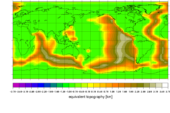
e_pot,th is shown in Fig. 2, and the resulting lithospheric stress field in Fig. 3. As should be expected, this part of the stress field is characterized by tensile stresses close to the ridges and compressive stresses elsewhere. Directions of of maximum compressive stresses tend to be parallel to ridges. Additionally, where two ridges are close to each other, but not actually connected (spreading ridge between Nazca and Cocos plates, and Mid-Atlantic ridge), they tend to be in the direction from one ridge to the other. The mean azimuth error is 35.19^°.

Topography h_c isostatically compensated within the crust.

It is assumed that h_obs-h_d-h_th is isostatically compensated in the lithosphere. For the given crustal model, we are able to compute which topography h_c would be isostatically compensated in the crust. The difference h_sc: = h_obs-h_d-h_th-h_c is assumed to be isostatically compensated within the lithosphere at subcrustal levels (see next section).

h_c is equal to , whereby is the amount by which the crust would need to be vertically displaced in order to be in isostatic equilibrium. is therefore given by

below air and

below water, whereby is the density of water and t_w is the thickness of the water layer; the constant is a posteriori determined such that h_c has a zero global mean value; z is counted positive upwards. For integration between the Moho and the surface of the solid Earth (including ice sheets) the crustal model is used. Below the Moho, a constant mantle density is assumed. With these assumptions, is independent of which z₀ is chosen as long as it is below the Moho depth everywhere.

After a change of integration variables, these equations are solved for and we obtain

below air and

below water, where h_sl is the height of the sea level, i.e. integration includes the water layer. Equations ``below air'' are used for h<sub>obs</sub> > h<sub>sl</sub> and ``below water'' for h_obs £ h_sl.

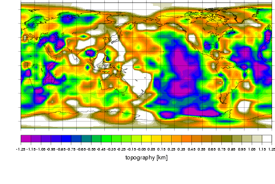
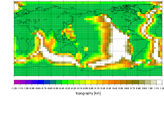
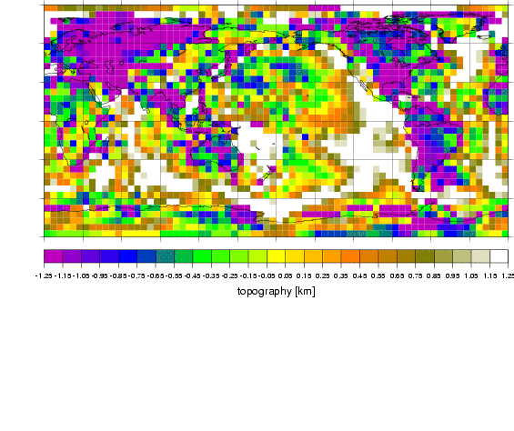
The topography not isostatically compensated within the crust is shown in Fig. 4. This figure clearly shows the oceanic ridges, but also the region between Australia and Tonga to be elevated. The continents, with the exception of Africa, tend to be depressed relative to the oceans. In Fig. 5 the effect of cooling of the oceanic lithosphere has been substracted, i.e. this figure shows . The spherical harmonic expansion of h_res up to degree 31 is shown in Fig. 3b of the main text and compared to h_d.

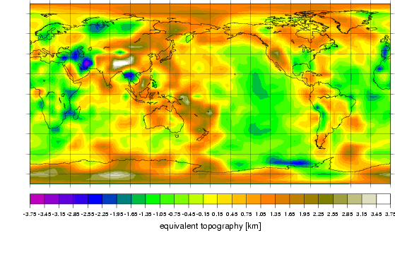
The potential energy per area of the isostatically compensated topography is therefore

below air and

below water. Qualitatively, these equations describe that mountains have the tendency to flow apart, as this would reduce their excess potential energy, hence they are under tension. e_0,c is again chosen such that the global mean value of energy is zero.

e_pot,c is shown in Fig. 6 and the resulting lithospheric stress field in Fig. 7. The mean azimuth error is 44.14^°, i.e. it is almost uncorrelated with the observed stress field. Again the result is not surprising, as this part of the stress field is characterized by tensile stresses on the continents, which tend to be particularly large in mountain ranges, and compressive stresses in the ocean basins. Directions of of maximum compressive stresses tend to be parallel to mountain ranges.

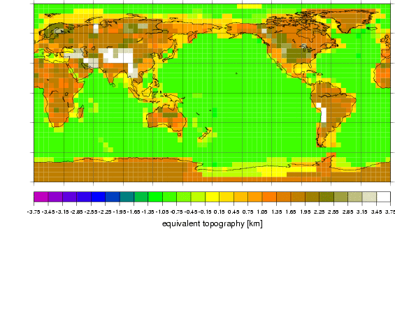
e_pot,c+e_pot,th is shown in Fig. 8 and the corresponding lithospheric stress field in Fig. 9. The mean azimuth error is 39.26^°.

Topography h_sc isostatically compensated below the crust.

For h_sc we choose as isostatic compensation the arithmetic mean of the Moho depth -h_Moho and 100 km (equivalent to assuming that isostatic compensation is equally distributed over the mantle part of a 100 km thick lithosphere), therefore the corresponding potential energy is

below air and

below water, with e_0,sc such that e_pot,sc has zero global mean.

h_sc is shown in Fig. 10, e_pot,sc is shown in Fig. 11 and the resulting lithospheric stress field in Fig. 12. The mean azimuth error is 46.97^°.

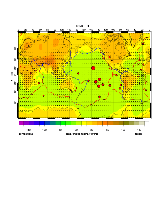
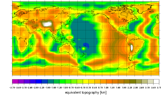
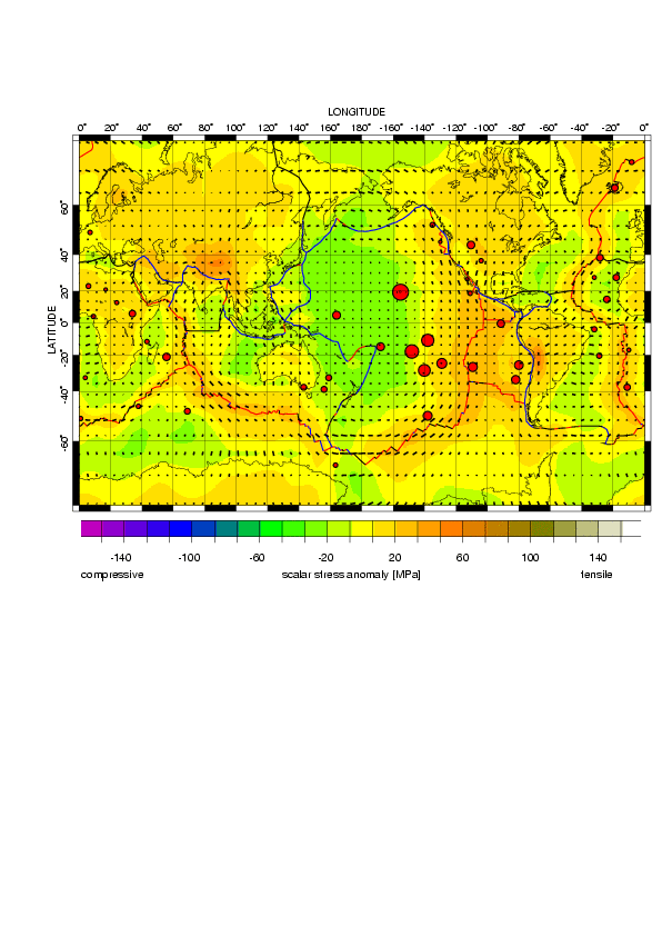
The potential energy of all non-dynamic topography e_pot,c+e_pot,sc+e_pot,th is shown in Fig. 13, and the resulting lithospheric stress field in Fig. 14: Calculated directions of maximum compressive stress bear no resemblance to the observed large-scale stress field (mean azimuth error 42.40^°, i.e. nearly uncorrelated) and hotspots appear both in regions with tensile and with compressive stress anomalies calculated. The poor fit of stress directions occurs, because we have substracted the assumed dynamic topography. If instead the dynamic topography is set zero (shown in Fig. 6, top right, of main text) the result is much better (only 30.37^° mean azimuth error).

References

B. Parsons, J.G. Sclater, An analysis of the variations of ocean floor bathymetry with age, J. Geophys. Res., 82 (1977) 803-827.

Figures

Figure 1: Topography due to ocean floor cooling, averaged on to a 5×5 degrees grid. Zero global mean; topography above 1.25 km is also shown in white.

Figure 2: Potential energy per area of topography due to ocean floor cooling, evaluated on a grid of 32 Gaussian latitudes and 64 points in longitude (suitable for spherical harmonic expansion) and linearly interpolated. The potential energy per area is expressed in terms of ``equivalent topography'' , with ``crustal density'', i.e. 1 m of ``equivalent topography'' corresponds to the potential energy of 1 m topography below air isostatically compensated at a Moho in 35 km depth.

Figure 3: Predicted lithospheric stress anomaly caused by topography due to ocean floor cooling. The contributions to lithospheric stress anomalies displayed in the figures of this background data are displayed in the same way as the total computed stresses in Figure 5 of the main text.

Figure 4: Topography not isostatically compensated within the crust on a 5×5 degrees grid. Zero global mean; topography above 1.25 km is also shown in white, below -1.25 km also in violet.

Figure 5: Topography not isostatically compensated within the crust minus topography due to ocean floor cooling on a 5×5 degrees grid. Topography above 1.25 km is also shown in white, below -1.25 km also in violet.

Figure 6: Potential energy per area of topography isostatically compensated in the crust, on a 5×5 degrees grid. It is again expressed in terms of ``equivalent topography''. Zero global mean; above 3.75 km is also shown in white.

Figure 7: Predicted lithospheric stress anomaly caused by topography isostatically compensated in the crust.

Figure 8: Potential energy per area of topography due to ocean floor cooling, plus topography isostatically compensated within the crust, evaluated on a grid of 32 Gaussian latitudes and 64 points in longitude (suitable for spherical harmonic expansion) and linearly interpolated, again expressed in terms of ``equivalent topography''. Above 3.75 km is also shown in white.

Figure 9: Predicted lithospheric stress anomaly caused by topography due to ocean floor cooling, plus topography isostatically compensated within the crust.

Figure 10: Topography not isostatically compensated within the crust minus topography due to ocean floor cooling minus dynamic topography expanded in spherical harmonics up to degree 31. Topography above 1.25 km is also shown in white, below -1.25 km also in violet.

Figure 11: Potential energy per area of topography h_sc, assumed to be isostatically compensated at a depth equal to the arithmetic mean of the Moho depth and 100 km, again expressed in terms of ``equivalent topography''. Above 3.75 km is also shown in white.

Figure 12: Predicted lithospheric stress anomaly caused by topography h_sc, assumed isostatically compensated at a depth equal to the arithmetic mean of the Moho depth and 100 km.

Figure 13: Potential energy per area of all non-dynamic topography expanded in spherical harmonics up to degree 31, again expressed in terms of ``equivalent topography''.

Figure 14: Predicted lithospheric stress anomaly caused by all non-dynamic topography.

5. Results for other tomographic models